
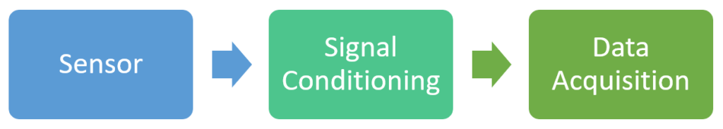
In this chapter we are talking about how the electric signal is converted to a digital signal so we can process it in a program. This conversion is called analog to digital conversion and before moving forward let’s discuss what analog and digital signals are.
Analog Signals
Analog signals are the signals which are present in real world. The voltage waveform present on the end of your wire is an analog signal, temperature is an analog signal, even more the voltage signal that carries digital signal information is an analog signal too.
To put it in a more scientific way analog signals are continuous in time and continuous in their codomain too.
- Continous in time: if you take two samples from the analog signal, let them be as close to each other as possible in time, there is still going to be other samples between them. Practically you can zoom into them on the time axis infinitely.
- Continous in codomain: if you take two samples from an analog signal and check their value, let them be as close to each other as possible in value, there are going to be other other values between them. Practically you can zoom into them on the amplitude axis infinitely.
Thinking about the points above we can easily get to an interesting conclusion: an analog signal has infinite amount of information.
Digital Signals
A digital signal represent an analog signal only in definite points in time, between these points we can only estimate what’s up with our original signal. In other words they are discrete.
Also a digital signal can represent only a certain set of values. It is incorrect to state that a digital signal can be either 1 or 0, that’s the characteristic of boolean values. A digital signal can represent 2^n type of values, where n is how many bits make a single digital value.
So the wires that carry the electric signal which represent a digital signal are also analog signals, their meaning is digital so the lesson here is that digital signals are a representation of various values and strictly speaking they only exists in software.

The other important conclusion is that digital signals carry a finite amount of information.
Analog to digital conversion thus means you take a finite amount of information from infinite amount of information. If you do it well you will keep sufficient enough information for your application and let the unimportant part go.
Analog to Digital Converters
Now we understand what is the input and the output of an analog to digital converter (or ADC), let’s see how they work.
The basic element of an ADC in theory is a comparator. It can be built from fairly simple electrical components (an operational amplifier) and has two inputs an one output. The function is also quite simple: if input 1 is lower than input 2 the output is low, if input 1 is higher than input 2 the output is high.
Well our theoretical ADC has lots of these comparators and input 1 where the signal to be converted is connected, input 2 is a reference voltage but it is different for each comparator. In the following video you can see how this works. The green LEDs represent the comparator outputs, the horizontal lines represent the decision level (treshold) for each comparator.
Let’s discuss a few things here:
- In this example there are 8 comparators, so can differentiate 8+1 signal levels. After this conversion we only know in which range the signal is (represented by the comparators) but we do not know any additional detail about the value itself.
- It is very important to mention that this example is not an 8 bit ADC. We will discuss this a bit later on but remember: in this example we can differentiate 9 different signal levels that can be represented on 4 bits so this would make this theoretical ADC a not fully 4 bit one.
The conversion itself takes some time so the conversion needs some timing.
Most important characteristics of ADCs
Sampling Rate
Sampling rate defines how many samples the ADC converts from the analog signal to a digital signal per second. The higher the sampling rate the lower the amount of time is available to sample the signal so the more difficult it is to take an accurate measurement/conversion.
In general your signal source defines the requirements for sampling rate. It doesn’t matter to take a 10 kS/s measurement on a temperature sensor in your living-room as it will definitely not change that fast, especially that your sensor won’t be able to follow changes that quickly. On the other hand if you want to see the waveform of the electric network in your house (50 or 60Hz) then it doesn’t make sense to use a 2 S/s measurement as it won’t be able to tell you the waveform itself.
The Nyquist-theorem (he was Swedish so his name should be pronounced properly as “kneekvist”instead of the commonly used “naighkvist”) says that for a sampling rate you should select the frequency which is twice as much of the frequency you want to measure. This is a requirement because of aliasing in the frequency domain. What you should remember is that sampling itself has a so called modulation effect in the frequency domain and if you are not sampling at least twice as fast as the frequency of your signal then you cannot tell properly the frequency of the original, analog signal.
- Top-left graph shows the original (analog) signal
- Top-right graph shows the sampled signal
- Bottom-left graph shows the spectrum (FFT) of the original (analog) signal
- Bottom-right graph shows the spectrum (FFT) of the sampled signal
What you can see here is how the spectrum changes as the sampling rate decreases. The frequency of the original signal is 25 Hz so the video is slowed down around 60 Hz sampling so it is visible what happens when we go below the Nyquist limit.
There are cases when we do Undersampling (sampling under the Nyquist limit) or Oversampling (taking way more samples than needed) on purpose. This is not discussed here, you can find more details by the Nyquist-Shannon theorem.
The Sampling Rate is often given in S/s (samples per second) or Hz.
Resolution
The resolution is practically the number of possible values in the digital signal’s codomain. The better resolution you have the more closely the digitized signal follows the values of the analog signal.
Let’s do some math related to resolution:
- Suppose our ADC is a 8 bit one so we can differentiate 2^8 = 256 different values
- If our input range is 10 V the smallest difference/step our ADC can measure is 1 / 256 * 10 = ~0.039 V = 39 mV. This is also often referred to as the LSB (Least Significant Bit) as the LSB in the ADC’s output represent this value.
- Your ADC only outputs decimal values (how many comparators’ treshold is crossed) thus to get the actual physical value you multiply the ADC output with 1/2^n * range (so the LSB).
We discussed at the Signal Conditioning chapter that it is important to match the sensor’s output to the ADCs input. Now let’s see why:
- In the example above we discussed that our ADC’s input range is 10V and has 8 bits resolution so the LSB is 39 mV
- Now suppose we want to digitize a 0..1 V sine signal. In this case the accuracy is 39 mV / 1 V = 3.9 % In other words in this case we are only using one tenth of the overall resolution.
- Now let’s suppose that we amplify our signal by 10x so it will also be 0..10V. In this case the accuracy is 39mV/10V = 0.39% so we improved our measurement accuracy by 10x because using the correct range.
Resolution though is not everything. The sensor, the cabling, the amplifiers, the ADC take on some electrical noise and this can be significant. Noise on the measurement is often described as the number of LSBs. This tells you how many LSBs you cannot trust because of the noise. This is sometimes also calculated as Effective Number of Bits (ENOB).
Let’s take a typical use-case for ADC specs: a computer soundcard. The two most important parameters you see in the specifications:
- 44100 Hz (or such) – This is the sampling rate. Using this rate you can capture audio signals up to 22’050 Hz according to the Nyquist-theorem. This is great for as as above 22’050 Hz you cannot hear sound anyway.
- 24 bit (or such) – This is the resolution. 24 bit is a relatively really good resolution and we need this for the appropriate dynamic range (so we can hear loud and low sounds too)
ADC Types
However the most straightforward way to implement an ADC is using multiple comparators there are other ways to do this. In the list below we discuss a few of the common ones.
Flash ADC
This is the one we practically already discussed – the theoretical ADC. It has many comparators and each comparator has its reference voltage created with the help of a resistance-ladder. As the conversion can happen in one iteration these ADCs are very fast and also quite expensive.
Delta-Sigma ADC
(also called Sigma-Delta) The operation of the Delta-Sigma ADCs is quite complex, it works via a process called modulation and then the modulated signal goes through a digital filter.
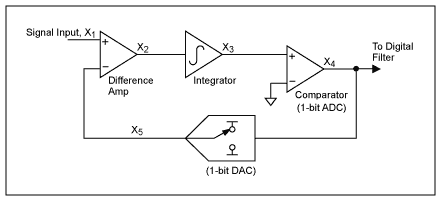
To put the long story short: these ADCs have an internal +/- voltage step defined. The analog signal is connected to the ADC’s input and the ADC tries to follow it by either subtracting or adding the internal voltage step to the input signal. Each time the the follower signal goes above the original signal a 1 is generated on the output of this element, each time it is under it a 0 is generated. This is not the final output of the digitizer but an internal variable and is generated very fast. A second element implements a digital filter and thus the final, digitized value is generated on the output. You can find more details here.
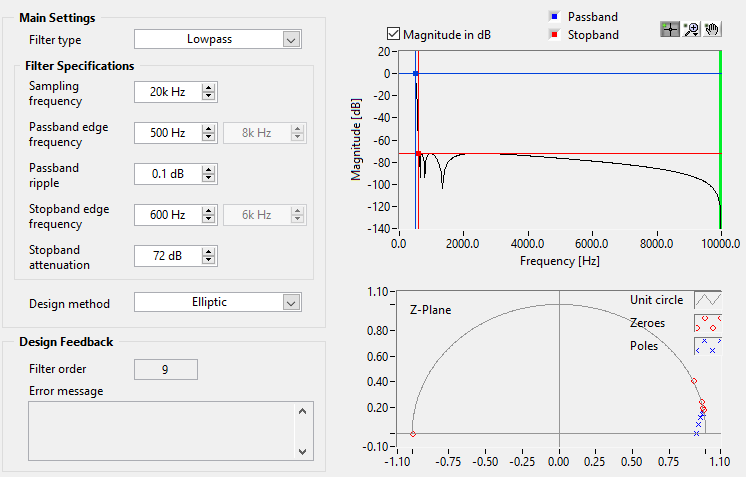
The picture above shows the digital filter settings that are used in the video example below. As you can see this is a 9th order Elliptic filter and the passband edge frequency (where it starts to cut-off) is at 500 Hz. This is selected as I am using a 20x oversampling and considering the Nyquist theorem.
What you can see in this video:
- Left-top-chart: the input signal (blue) and the internal signal (red) that “tries to follow” the input
- Right-top-chart: the input signal (blue) and the internal digital signal (right) that is practically the output of the 1 bit ADC.
- Left-bottom-chart: the output of the virtual ADC visualized
Successive Approximation ADC
Successive Approximation (SAR) ADCs work in a way similar to how you try to find the burnt light bulb in the Christmas lights. If your Christmas light strip doesn’t work the fastest way to find the burnt bulb is the following: remove the bulb in the middle and check which side’s resistance is infinite thus you know the burnt bulb is in that half. Now repeat the same process for the broken half of the light strip. And repeat over to the one bulb that is broken.
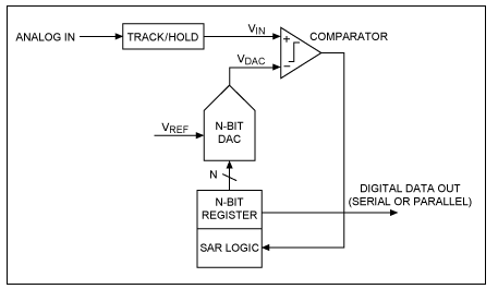
SAR ADCs work is a very similar way: check if the input value is higher or lower than the middle of the range – the reference signal that changes in each step. Then do the same for the range that contains the signal based on the previous step and repeat over the process for N iterations. The more iterations you have the closer you get to the actual value and your output will be practically the reference signal’s value. As this process needs to happen for every single value you need to run it very fast.
The video above shows the differences between iterating 1..8 times in the SAR ADC.
- Chart on top-left shows the input signal (blue) and the reference signal (red). For better visibility the iterations in the reference signal are also plotted against the time while showing the input value being samples. This is the reason having steps in the input signal.
- Chart on top-right shows the input signal (blue) vs the digitized signal (red). Of course the closer they are the better the digitizer is.
- Chart&table on bottom-right shows the accumulated squared error values (signal-digizited value)
- Slider on the bottom-left shows how many iterations are being used in the digitizer.
How good the measurement is?
The two keywords are measurement and accuracy. These are often explained via throwing darts however I thinks this is not straightforward as it is not correlated to how it works in reality. Let’s start with what can make our measurements incorrect.
- Random errors: it means that the digitized value is always “around” the real value within a certain deviation. In most cases these errors are coming from electric noises on the cables, temperature noises in components and such. The less random error you have the more similar your samples will be on the same input value so the more precise your measurement is.
- Systematic errors: in certain cases the measurement errors show some pattern so they can be predicted and thus corrected. A typical systematic error is an offset error that can be the result of incorrect coupling or having a bias in the signal, temperature drifts and such. Knowing the measurement setup or doing statistics on the digitized signal you can calculate the offset and remove it from the measurements. If the systematic errors are minimal (or removed) and your have a good precision then your measurement is accurate. So the value you are measuring is the value of the real, analog signal.