
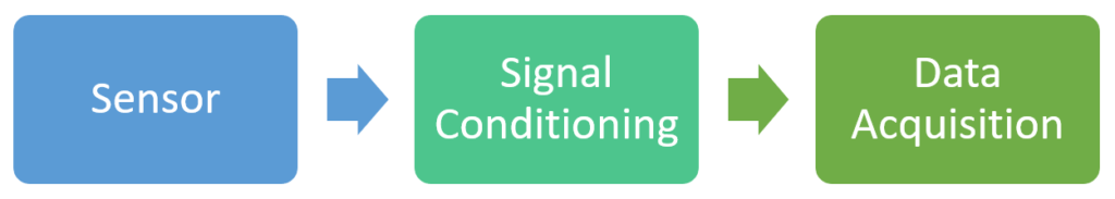
It is important to recall that the highest amount of information is right on the sensor and with every step in the measurement chain we loose some, although to goal is to minimize the loss. Elements in the measurement chain cannot restore lost information but can form the signal so that we can extract the information important for us.
Information flow
Output of the Signal Conditioning element
At the end of the day we can measure voltage in the data acquisition phase. Of course in rare cases there are other type of electric signal we can connect to an Analog to Digital Converter but in the vast majority of cases it is voltage we want as an output of the signal conditioning phase.
X2V (Whatever to Voltage)
Sensors that doesn’t output voltage need signal conditioning so that their output can be connected to the data acquisition device.
Resistance Output Sensors
To convert a resistance to voltage you simply need to run current through it. The difficult part is to create a precise constant current generator, as changes in the current appear as changes in the measure voltage too. R*I = U so there is a linear relation between the current changes and the voltage changes.
To overcome this challenge you either use a precise and expensive current source or create a voltage divider and hook up your circuit to a voltage divider. Voltage dividers help in a way that the ratio of the two resistors define the output voltage. However they are still sensitive to the changes in the supply voltage it is not a big deal as it is relatively easy to make a stable voltage source.
One more step forward is ratiometric measurements where you compare the output of two voltage dividers connected to the same voltage source so they are not sensitive to even voltage supply changes. The most famous of those is the Wheatstone bridge, often used in strain-gauge measurements.
Current Output Sensors
Converting current to voltage is very easy, you let the current flow through a resistance (which in this case is called a Shunt) and measure the voltage.
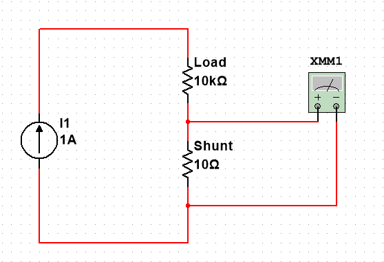
However keep in mind that the current going through the Shunt is generating some heat that needs dissipation. A low current with low Shunt is perfectly OK to use but you don’t want to put a Shunt on 10 Amps.
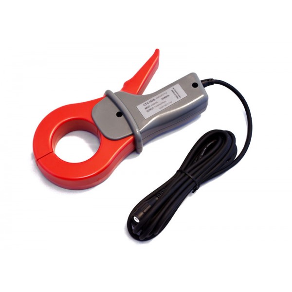
In this case the good choice is a Current Clamp which uses the Hall effect to measure the current flowing in the wire the clamp is placed on. Of course a current clamp doesn’t need to look like a real clamp, you can find PCB mountable options too.
In process automation they often use so called transducers that measure something (pressure for example) and convert it to current. Practically current in this case also functions as the communication protocol. These are called 4..20mA interfaces where you simply scale the measured current to the real physical value. It starts from 4mA instead of 0 mA so that an open circuit can detected (this improves safety). These devices are usually measured via a Shunt.
IEPE Current Excitation
IEPE sensors are the ones that have a small circuit integrated into them so they amplify the charges generated by the sensor. These integrated circuits need a small amount of current as a supply and it is going through the same wires like the measurement itself.
Capacitance Output Sensors
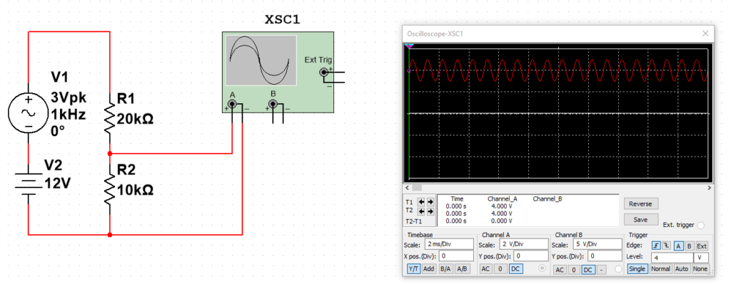
The easiest way to measure capacitance is to connect the device to a sine voltage source in series with a resistor and the capacitance changes will be visible as voltage changes. Of course there are more sophisticated methods too using amplifiers and such.
Coupling
When measuring a voltage you can select between AC and DC coupled measurements.
DC coupled measurements are the normal ones, so you measure the signal with all frequency components.
AC coupled measurements are the ones where you remove the DC components from your signal (so the low frequency components) and you only measure the AC components. Practically it means that you will see the changing parts of your signal but not the constants, it removes offsets. This is very often used for example in microphone measurements.

Scaling
The voltage range of the signal to be measured and the input voltage range of the data acquisition device might be different and you need to scale the signal to have the best match with input range – we will discuss the reason in the data acquisition part in details.
In case the signal to be measured is the higher you can divide it with a voltage divider. Of course if the signal range is 10’000 Volts and the input range is 5V you are not going to simply divide it, but in most cases of IoT applications a simple voltage divider can be great.
If the signal voltage level is too small compared to the input voltage range you need to amplify it with an amplifier circuit to have an appropriate level of details in your signal. Be careful though with this part because an amplifier can ruin your signal if incorrectly used and you really need a holistic view here.
In the video above you can see how the number of differentiated values (resolution) changes if we modify the gain of the input signal while the input range and conversion resolution remains the same. For example your sine signal is described with 255 type of values if it matches the full input range, but is described with ~50 type of values when it is only one fifth in amplitude of the input range.
Let’s say that you are measuring a thermocouple’s 40mV input but the measurement cables are not very well shielded and it introduces a ’30mV noise in the signal. So let’s amplify by 100x and you will have a 4V signal which is easy to process. Or is it? What we shall not forget is that in this case you will also amplify the 30mV noise so you will have a 3V noise on a 4V signal, not too great right?
A good workaround is to clear, filter your signal as much as possible before amplifying it and you do that with
Filters
Filters are special circuits that remove defined frequency ranges from your signal. Do we generate more information in your signal? No, but we remove the information that is not important, even more malicious for us.
Fourier’s theorem says that every periodic signal can be assembled from a series of sine and cosine signals with various multipliers. This is a beautiful topic and once I will explore it in a blog post. For now: this theorem also works with non-periodic signals even if not in a perfect way. Also sine and cosine means here that sine components that are in phase with the original signal and components that are 90 degrees shifted (this is called quadrature). The beauty here is how well you can manipulate these components with electric circuits and how well it is awarded in the resulted signal. Some proof that the theorem is true:
Analyzing the frequency components of a signal is called Fourier transformation and the result tells you what frequency components are there in your signal. We often use this representation (called frequency-domain) as it makes fairly simple to talk about filters and such instead of the time-domain representation. In the video above we created a square wave from 24 frequency components. Now let’s see its spectrum.

What can we tell from this spectrum?
- Each peak is representing a major frequency component in the original signal. There are 24 of them so our program works correctly as we assembled our square wave from 24 components
- The first peak is the base frequency, it can be read from the X axis that it is 10 Hz and you can tell from the Y axis that this is the most powerful one.
- The additional peaks are called harmonics as you can see they are at 3x, 5x 7x, 9x, etc.. the base frequency. This is how you construct a square wave.
- If we had only one peak at a time at the 10, 30, 50, etc… Hz frequencies then we would have 10, 30, 50, etc… Hz sine waves but now that we have all of them at the same time they make a square wave (this is what the video shows)
- This is a software generated square signal so it is quite clear. In real life there would be way more noise between the peaks. Also DC components (ones around 0 Hz) would appear so it can be tricky: not necessarily the lowest frequency peak in the spectrum is your base frequency.

I have added a 0.05V uniform noise on the 1V square wave signal and now compare the spectrum with the clean one. This is more lifelike and shows why is it important to do proper filtering. (uniform noise means that it is evenly distributed over the spectrum)
When using filters you are using your a priori knowledge of a signal and remove the parts that you don’t want to measure. A good example is the noise coming from the electric network. Just connect a piece of wire to the measurement device and leave the other end floating. If the measurement device is fast enough one of the main components you will see in the signal is the 50 or 60 Hz component (depending on where you are in the world). This component can be filtered out with a high-pass (leaving the components in the signal above 50Hz) or band-stop filter (only removing the close environment of 50 Hz components). An other good example is the 13 Hz filters applied on ECG signals to remove ECG noise coming from human muscle contraptions. But again: no signal improving magic here! By removing certain frequency components you also remove these components not just from the noise but from your actual signal too – so for example the square wave will not be that nice. Why we still do this is the trade-off: by thoroughly understanding your signal you can gain more with removing a noise component that loosing by removing a certain part of the signal itself.
Also you cannot remove just the 50 Hz component but you will remove frequencies close to it, also not equally but with a certain multipliers. Filter designing is a whole profession and if you are interested you can read more about it on the internet or play with it here.
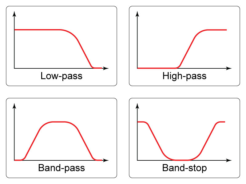
Depending on what you want to accomplish you can choose from 4 basic filter types. The diagrams represent the amplitude vs frequency. So where the curve is high the frequencies can get through the filter and where it is low the frequencies are blocked in the filter.
In the next video we add noise to a 200 Hz sine signal and amplify it. In case of the white signal we apply a band-pass filter before the amplification. The band-pass filter is tuned around the 200 Hz range. What can be examined here is that even with a huge noise the original sine signal can be reconstructed very well.
The two commonly used, simple filters: low-pass and high-pass filters can be realized with a capacitor and a resistor and you can find the details here.
We are going to discuss more about filters and spectrum in additional blog posts in the future.